Diffusion in Zeolites
Difficulty: Medium
Summary
Zeolites, which have complex cage structures of silica and aluminium, are extremely important in industrial catalysis. In this exercise, the diffusion of an aromatic compound (benzene) in a model zeolite is studied, see . Diffusion rates are extremely slow in these systems, so a simple trick will be employed to attempt to improve matters.
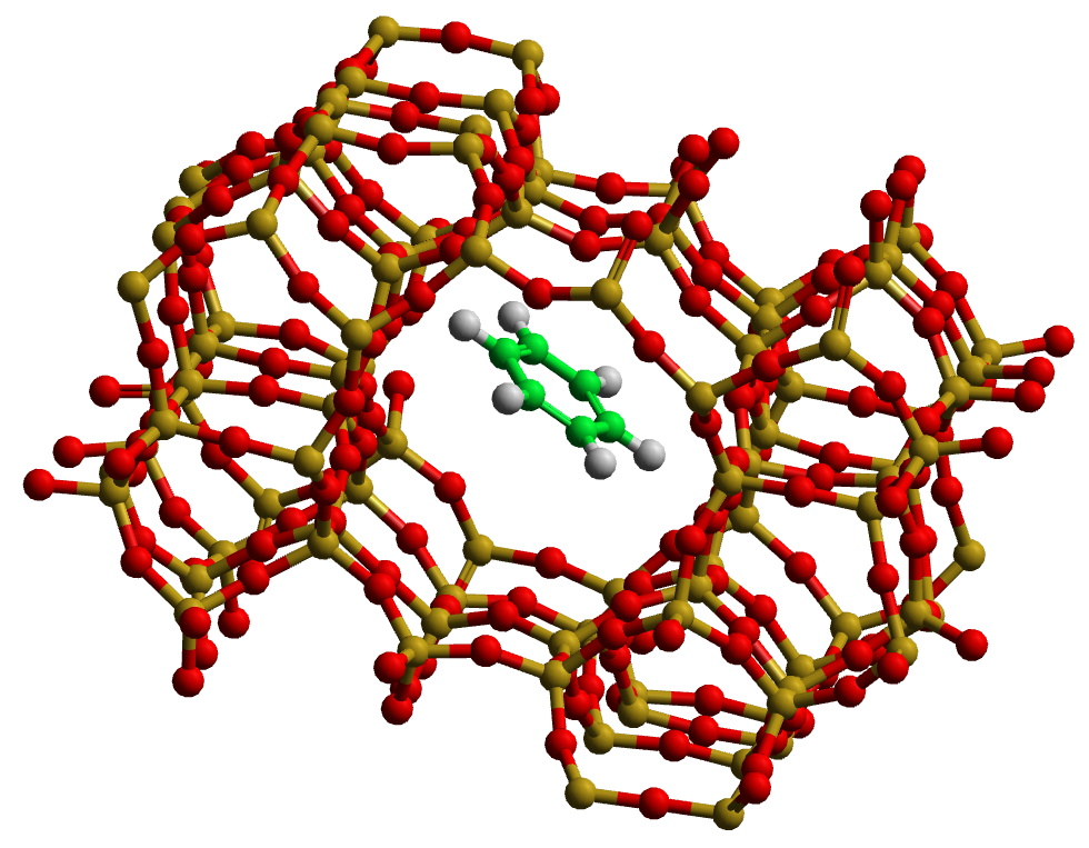
Zeolite cage with a benzene molecule trapped inside
Background
In this exercise the silicalite-1 structure is used as a model for the zeolite ZSM-5, which has application in synthesizing stereospecific aromatic derivatives. The process has (at least) two aspects to it: firstly the aromatic species must diffuse into the zeolite and secondly it must undergo catalytic reaction within the confines of the zeolite cages. (It is believed that the confinement within the cages is responsible for the sterospecificity of the reactions.)
Classical simulation cannot study the reaction process, but it is (usually) well suited to model the diffusion. The problem in this case however is that the diffusion is slow and it is difficult to get accurate estimates of the diffusion constant. There are a number of ways this can be overcome, perhaps the most promising of which is to use constraint dynamics (see exercise [ex:pmf]) to obtain the activation energy and feed this into a numerical model of the diffusion, ref [Forester1997], this however is beyond the scope of these exercises. Instead we shall employ a less rigorous approach, that has been used in studies of diffusion in amorphous polymers, ref [Plathe1991]. In this it is assumed that diffusion is governed by Arrhenius like behaviour:
where \(E_A\) is an activation energy and \(λ\) is a scaling factor between 0 and 1. The origin of the activation energy lies in the intermolecular interactions, and thus the factor \(λ\) is a control parameter governing the strength of these. We hope that by reducing the intermolecular interaction, we may effectively increase the measured diffusion constant \(D(λ)\) and later obtain the true diffusion constant (which corresponds to the case where \(λ = 1\)) by extrapolation.
Instructions
Copy the Exercise6.tar.xz file into the $DL_POLY/data directory and unpack:
cd $DL_POLY/data
wget https://ccp5.gitlab.io/dlpoly/Exercise6.tar.xz
tar -xvf Exercise6.tar.xz
Now go to the $DL_POLY/execute directory and start up the GUI:
cd $DL_POLY/execute
java -jar ../java/GUI.jar &
Task
Copy the contents of the subdirectory Exercise6 into the execute subdirectory. To do this using the GUI, select from the main menu Execute > Store/Fetch Data and in the Data Archive window type Exercise6 in the Fetch box and click Fetch. The CONFIG file contains a silicalite framework and a benzene molecule inserted into one of the cavities. The FIELD file contains the appropriate description of all the interactions (note this is a stripped down forcefield constructed for the workshop, and is not guaranteed for other uses!) Proceed as follows:
Use the GUI to visualise the original configuration. If you are not familiar with zeolite structures, it will be interesting for you to see what this one looks like! The structure is characterised by large inteconnecting cavities forming channels for the diffusion of penetrant molecules.
Run, see , a simulation for about 2000 timesteps, creating a HISTORY file. To save disc space, you should dump configurations only every 10 timesteps and should not dump atomic velocities at all. Use the MSD facility within the GUI to show the mean square displacement. Estimate the diffusion constant. It will give you an idea of what you are up against.
Edit the FIELD file using your favourite editor, reducing the strength of the interaction between the benzene and zeolite by some factor \(λ\) with \(0< λ < 1\) (this will involve Van der Waals terms only) and repeat the simulation to obtain the MSD and diffusion constant again. Do this at least two more times. (Note each simulation may take up to an hour.)
Plot the log of the diffusion constants against the parameter \(λ\). Can you estimate the diffusion constant at \(λ=1\)? How does it compare with your first run?
In each simulation you should look at the REVCON files produced by the DL_POLY run and see where the benzene has ended up. If it has changed channels in the zeolite, what effect do you think this might have on the the study overall? Try to form an opinion on how useful this approach is likely to be as a general technique.
Müller-Plathe, Diffusion of penetrants in amorphous polymers: A molecular dynamics study, The Journal of Chemical Physics, 94(4), p. 3192, 1991, doi: http://dx.doi.org/10.1063/1.459788
Forester and W. Smith, Bluemoon simulations of benzene in silicalite-1 prediction of free energies and diffusion coefficients, J. Chem. Soc., Faraday Trans., 93, p. 3249, 1997, doi: 10.1039/A702063E